Installation
The easiest way to get mlbplotR is to install it from CRAN with:
install.packages("mlbplotR")To get a bug fix or use a feature from the development version, you can install the development version from GitHub with:
# install.packages("devtools")
devtools::install_github("camdenk/mlbplotR")
Examples
Let’s plot every team on a grid with some extra customization:
library(mlbplotR)
library(ggplot2)
library(dplyr)

teams_colors_logos <- mlbplotR::load_mlb_teams() |>
  dplyr::filter(!team_abbr %in% c("AL", "NL", "MLB")) |>
  dplyr::mutate(
    a = rep(1:6, 5),
    b = sort(rep(1:5, 6), decreasing = TRUE),
    # Keep alpha == 1 for teams that have an "A"
    alpha = ifelse(grepl("A", team_abbr), 1, 0.75),
    # Set teams that have an "E" to black & white
    color = ifelse(grepl("E", team_abbr), "b/w", NA)
  )


 ggplot2::ggplot(teams_colors_logos, aes(x = a, y = b)) +
   mlbplotR::geom_mlb_logos(aes(team_abbr = team_abbr,
                                color = color, alpha = alpha),
                            width = 0.075) +
   ggplot2::geom_label(aes(label = team_abbr), nudge_y = -0.35, alpha = 0.5) +
   ggplot2::scale_color_identity() +
   ggplot2::scale_alpha_identity() +
ggplot2::theme_void() 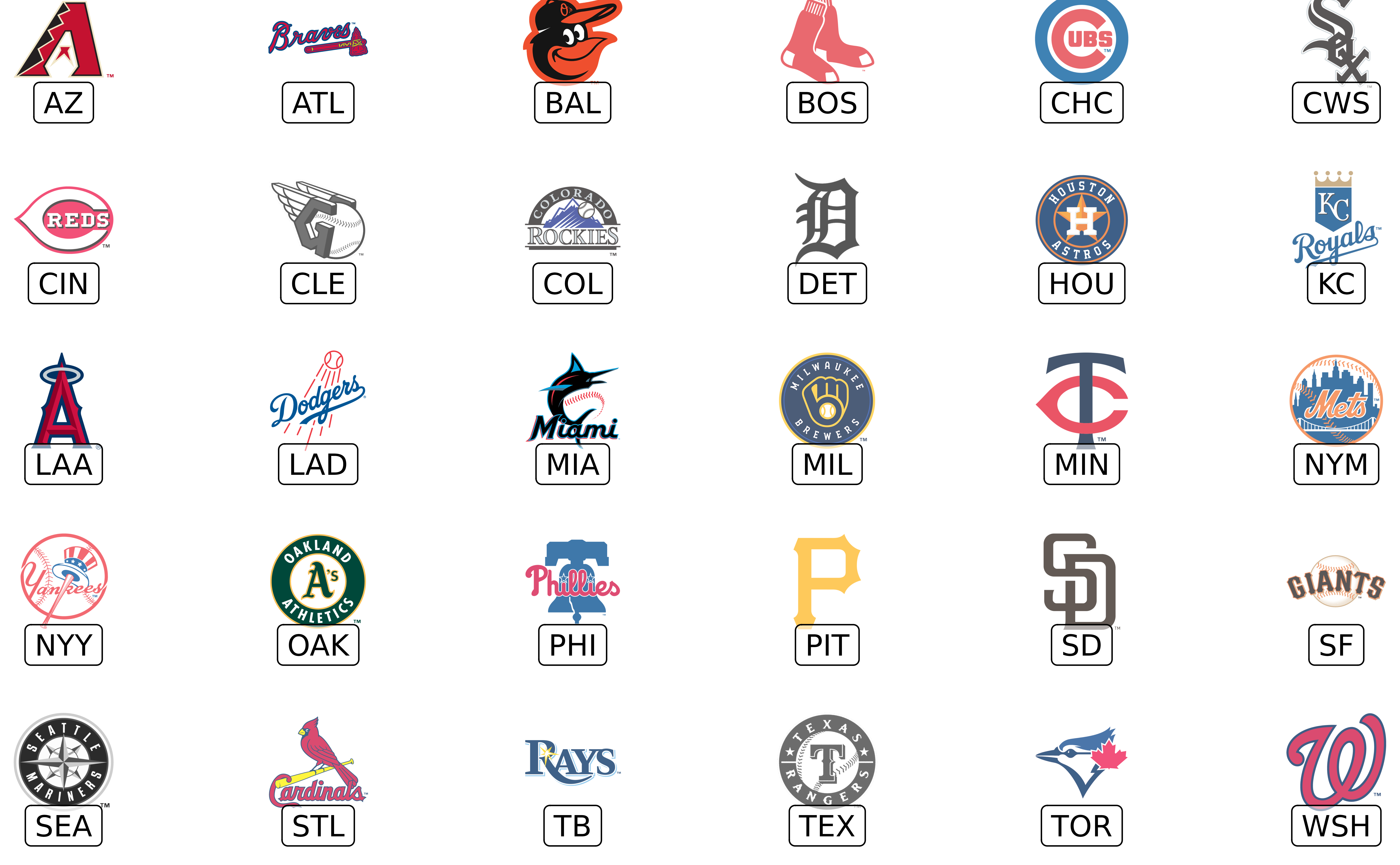
This is a basic example with FanGraphs data (pulled using baseballr) which compares ERA to FIP for each team’s top starting pitcher by ERA:
# Uncomment this to pull data, currently commented out to save
# a dependency on baseballr
#
# library(baseballr)
#
# df <- baseballr::fg_pitcher_leaders(x = 2021, y = 2021,
#                                     q = 100, pitcher_type = "sta")
#
# filtered_df <- df |>
#   dplyr::filter(Team != "- - -") |>
#   # FanGraphs Team abbreviations aren't the standard
#   # for what's used in the plotting functions so
#   # you could clean them with the following line,
#   # but the geom_*_logos() functions should all
#   # clean the abbreviations before plotting
#   #
#   # dplyr::mutate(Team = clean_team_abbrs(Team)) |>
#   dplyr::group_by(Team) |>
#   dplyr::slice_min(ERA, n = 1) |>
#   dplyr::ungroup()

library(scales)

filtered_df |>
  ggplot2::ggplot(aes(x = ERA, y = FIP)) +
  mlbplotR::geom_mlb_logos(aes(team_abbr = Team), width = 0.075, alpha = 0.7) +
  ggplot2::labs(title = "2021: ERA vs. FIP",
                subtitle = "Each Team's Top Starter By ERA | Min. 100 IP",
                caption = "Data: FanGraphs via baseballr") +
  ggplot2::theme_minimal() +
  ggplot2::theme(plot.title = ggplot2::element_text(face = "bold")) +
  ggplot2::scale_x_reverse(breaks = scales::pretty_breaks(),
                           labels = scales::number_format(accuracy = 0.01),
                           expand = c(.1, .1)) +
  ggplot2::scale_y_reverse(breaks = scales::pretty_breaks(),
                           labels = scales::number_format(accuracy = 0.01),
                           expand = c(.1, .1))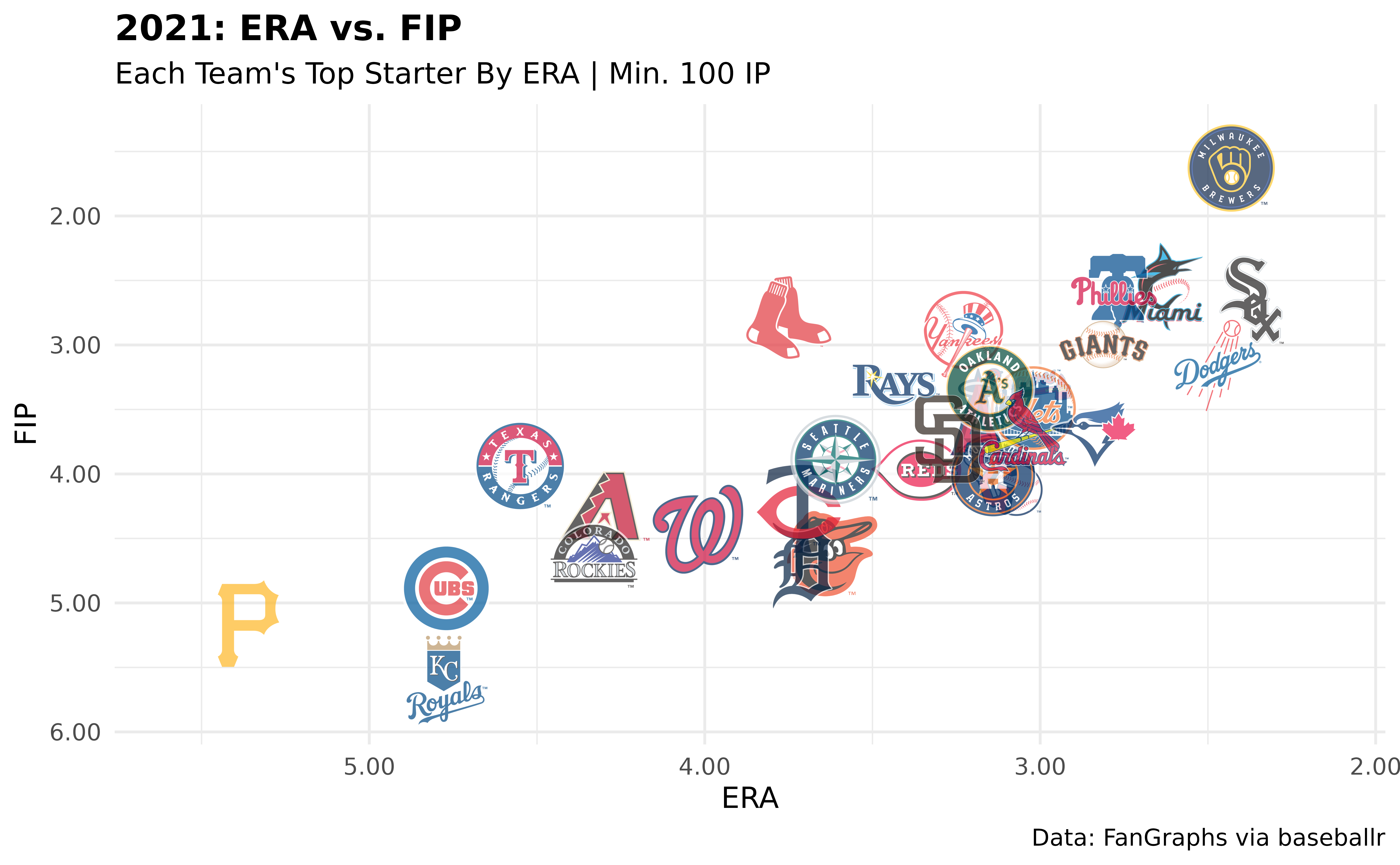
Here’s another that looks at Home Runs Allowed by top pitchers:
filtered_df |>
  # The scale_*_mlb() functions don't auto-clean abbreviations
  dplyr::mutate(Team = clean_team_abbrs(Team)) |>
  ggplot2::ggplot(aes(x = Team, y = HR)) +
  ggplot2::geom_col(aes(color = Team, fill = Team), width = 0.5) +
  mlbplotR::geom_mlb_logos(aes(team_abbr = Team), width = 0.07, alpha = 0.9) +
  mlbplotR::scale_color_mlb(type = "secondary") +
  mlbplotR::scale_fill_mlb(alpha = 0.4) +
  ggplot2::labs(title = "2021: Home Runs Allowed For Top Pitchers",
                subtitle = "HRs Allowed By Each Team's Top Starter By ERA | Min. 100 IP",
                caption = "Data: FanGraphs via baseballr") +
  ggplot2::theme_minimal() +
  ggplot2::theme(plot.title = ggplot2::element_text(face = "bold"),
                 axis.title.x = ggplot2::element_blank(),
                 axis.text.x = ggplot2::element_blank(),
                 panel.grid.major.x = element_blank()) +
  ggplot2::scale_x_discrete(expand = c(0.05, 0.075))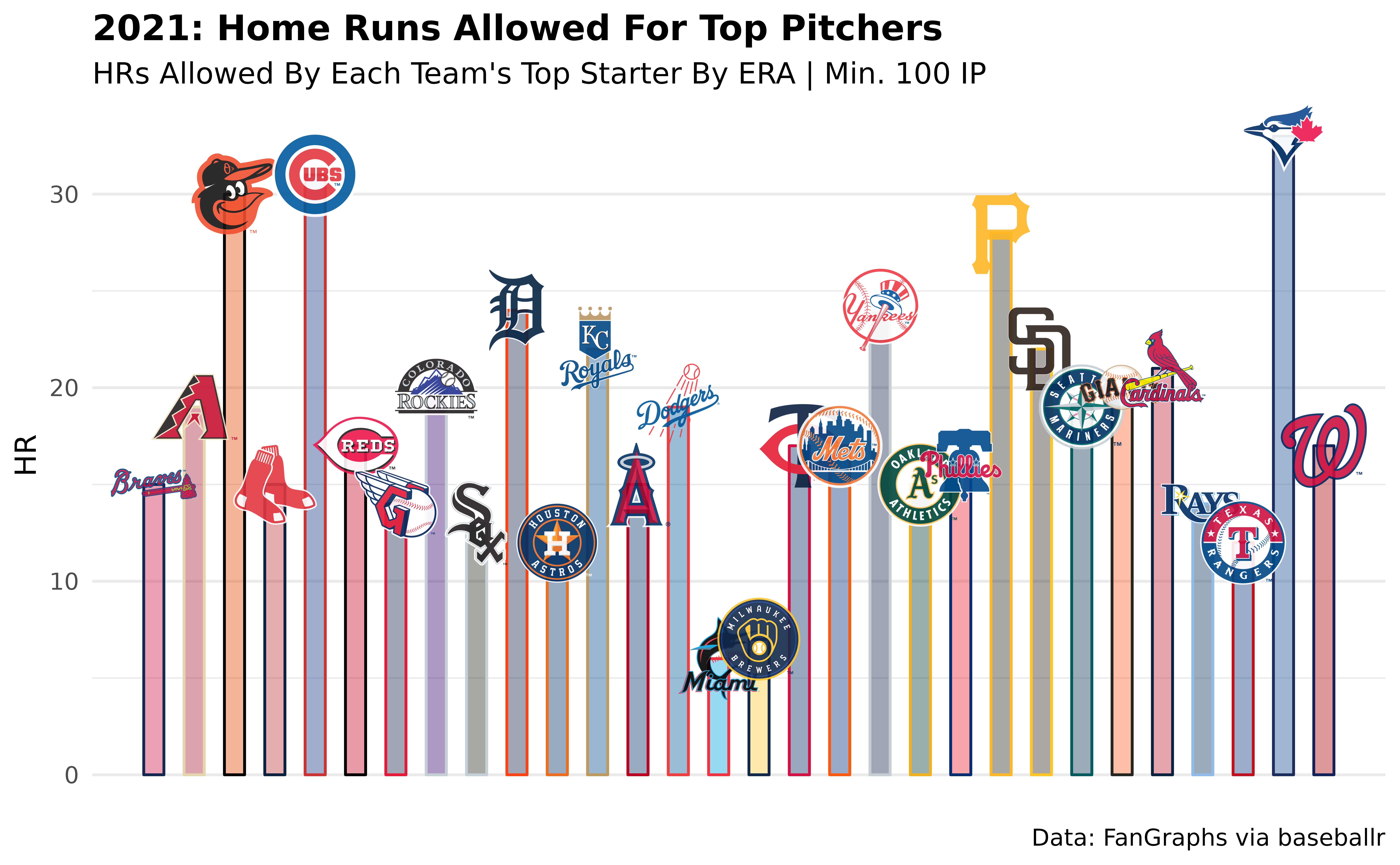
Instead of putting the logos in the plot, we can have them be the axis labels:
filtered_df |>
  # The scale_*_mlb() functions don't auto-clean abbreviations
  dplyr::mutate(Team = clean_team_abbrs(Team)) |>
  ggplot2::ggplot(aes(x = Team, y = HR)) +
  ggplot2::geom_col(aes(color = Team, fill = Team), width = 0.5) +
  #mlbplotR::geom_mlb_logos(aes(team_abbr = Team), width = 0.07, alpha = 0.9) +
  mlbplotR::scale_color_mlb(type = "secondary") +
  mlbplotR::scale_fill_mlb(alpha = 0.4) +
  ggplot2::labs(title = "2021: Home Runs Allowed",
                subtitle = "HRs Allowed By Each Team's Top Starter By ERA | Min. 100 IP",
                caption = "Data: FanGraphs via baseballr") +
  ggplot2::theme_minimal() +
  ggplot2::theme(plot.title = ggplot2::element_text(face = "bold"),
                 axis.title.x = ggplot2::element_blank(),
                 panel.grid.major.x = ggplot2::element_blank(),
                 # this line triggers the replacement of team abbreviations with logos
                 axis.text.x = mlbplotR::element_mlb_logo()) +
  ggplot2::scale_x_discrete(expand = c(0.05, 0.075)) +
  ggplot2::scale_y_continuous(expand = c(0, 0, 0.05, 0))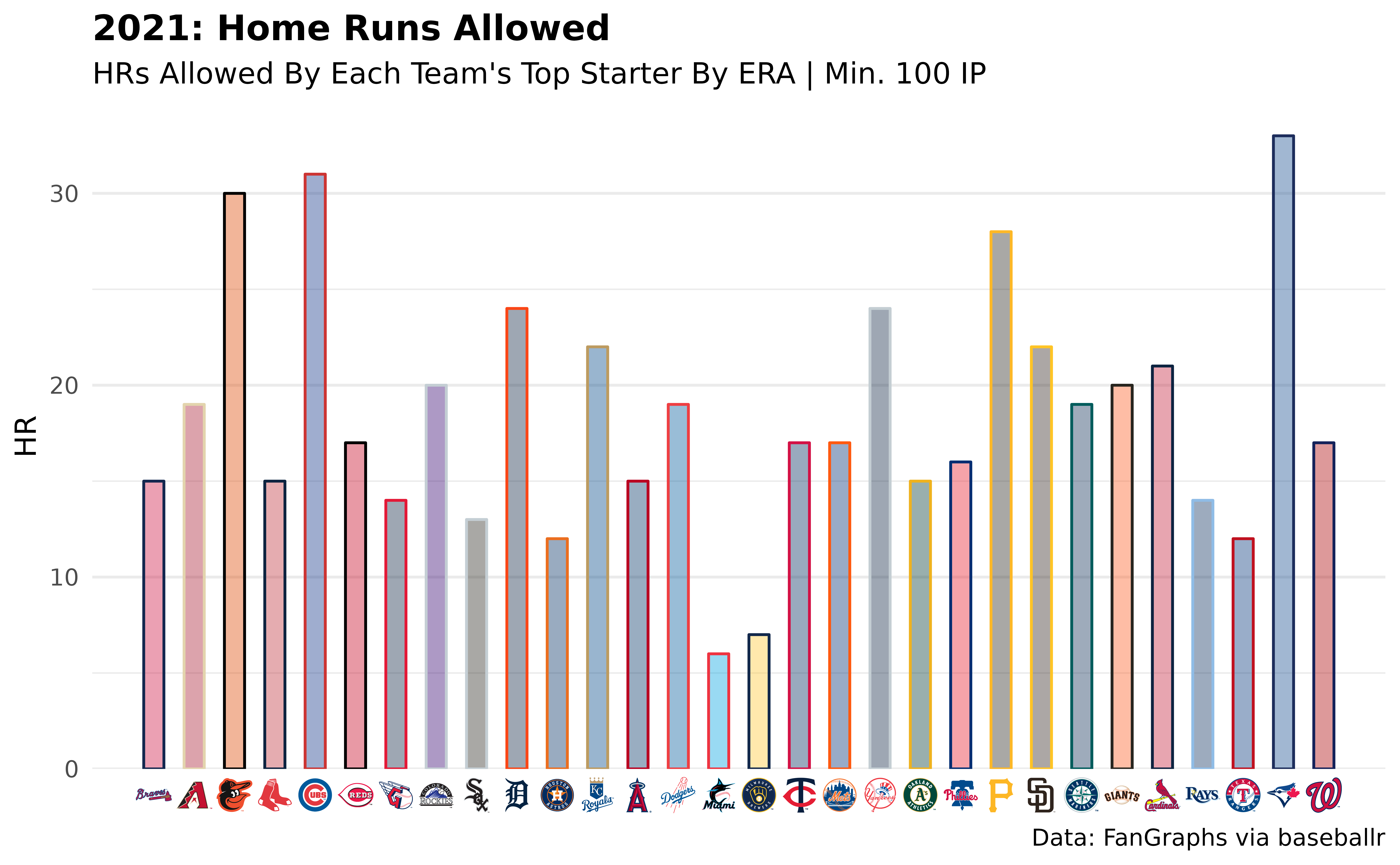
The family of element_*() functions allows for a lot of
extra customization with axes labels and can even be used for
facet_wrap()/facet_grid() strip headers.
Lastly, here’s an example using headshots:
# top_12 <- df |>
#   dplyr::mutate(playerid = as.double(playerid)) |>
#   dplyr::slice_min(ERA, n = 12)

top_12 |>
  dplyr::left_join(mlbplotR::load_headshots(),
                   by = c("playerid" = "fangraphs_id")) |>
  ggplot(aes(x = ERA, y = FIP)) +
  mlbplotR::geom_mlb_headshots(aes(player_id = savant_id), height = 0.15) +
  ggplot2::scale_x_reverse(breaks = scales::pretty_breaks(),
                           labels = scales::number_format(accuracy = 0.01),
                           expand = c(.1, .1)) +
  ggplot2::scale_y_reverse(breaks = scales::pretty_breaks(),
                           labels = scales::number_format(accuracy = 0.01),
                           expand = c(.1, .1)) +
  ggplot2::labs(title = "2021 SP ERA Leaders",
                subtitle = "Minimum 100 IP",
                caption = "Data: FanGraphs via baseballr") +
  ggplot2::theme_minimal() +
  ggplot2::theme(plot.title = ggplot2::element_text(face = "bold"))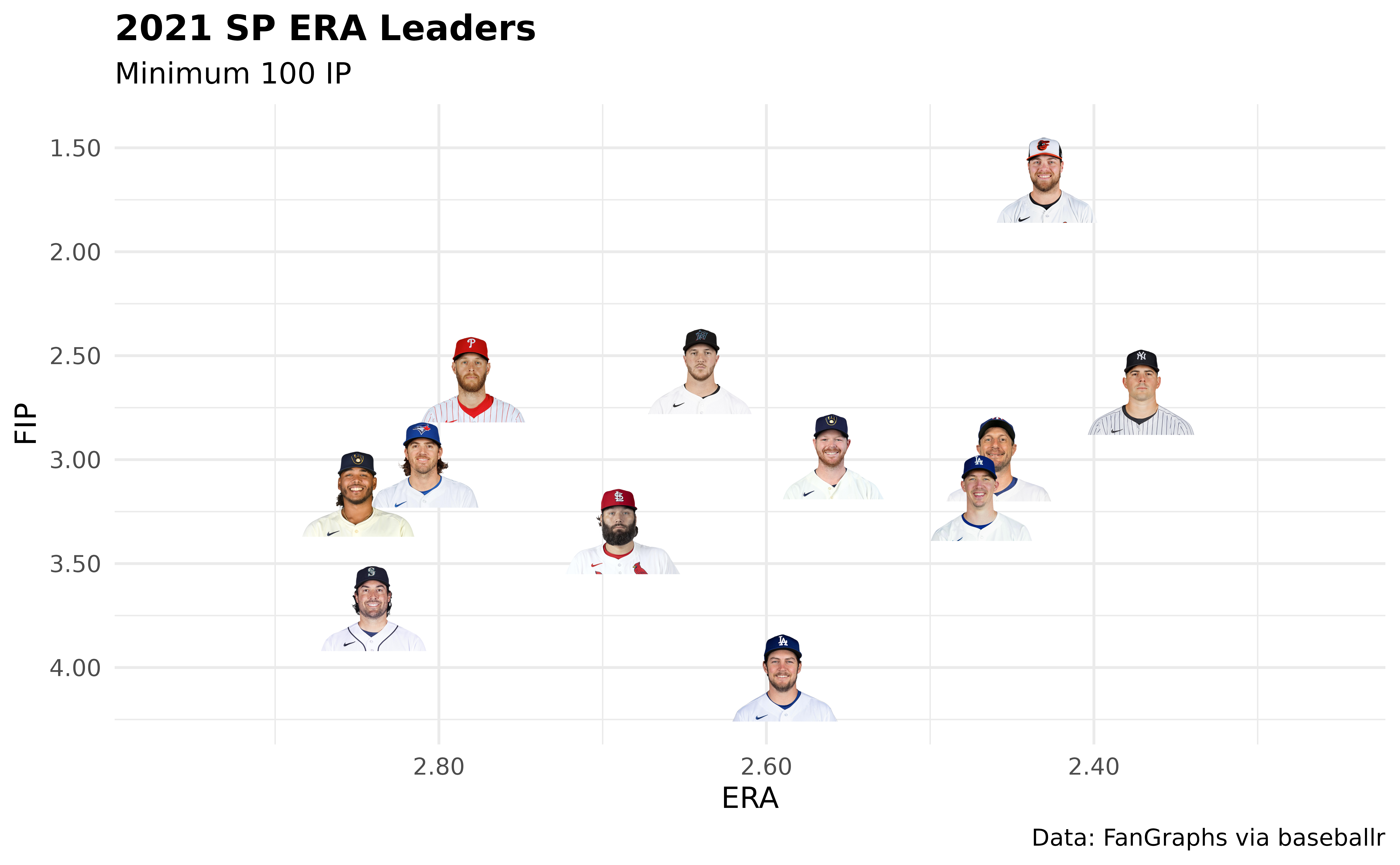
Note: If a player’s headshot data can’t be found, their headshot will be replaced with the MLB logo by default.
